Lecture 3: Experimental design

Causal Inference and Statistical Designs · Michaelmas 2026 · Qingyuan Zhao

Principles of experimental design

In The Design of Experiments (1935), Fisher suggested three principles:

  1. Randomization: The random assignment of treatments to experimental units.
  2. Replication: The repetition of an experimental treatment across multiple independent experimental units.
  3. Blocking: The grouping of similar experimental units into homogeneous blocks before assigning treatments randomly within those blocks.

We will discuss four experimental designs:

1. Blocking, 2. Stepped wedge, 3. Group sequential, 4. Enrichment.

Covariate adjustment for completely randomized experiments

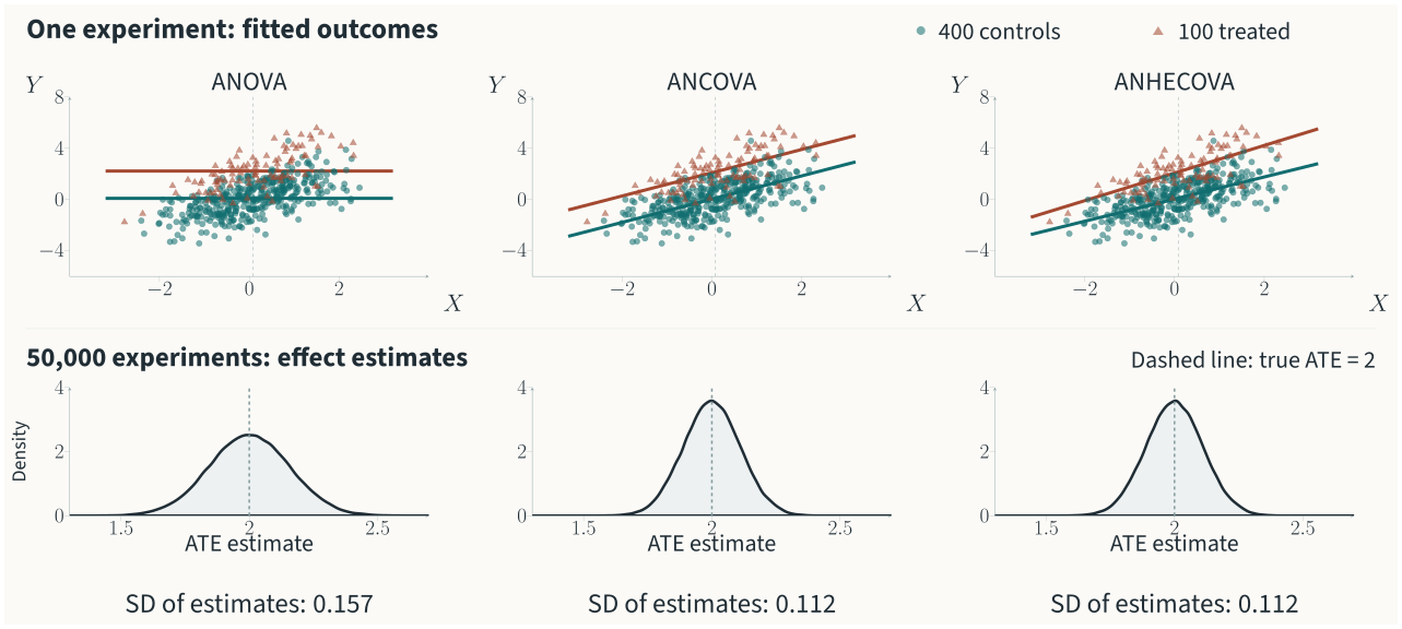
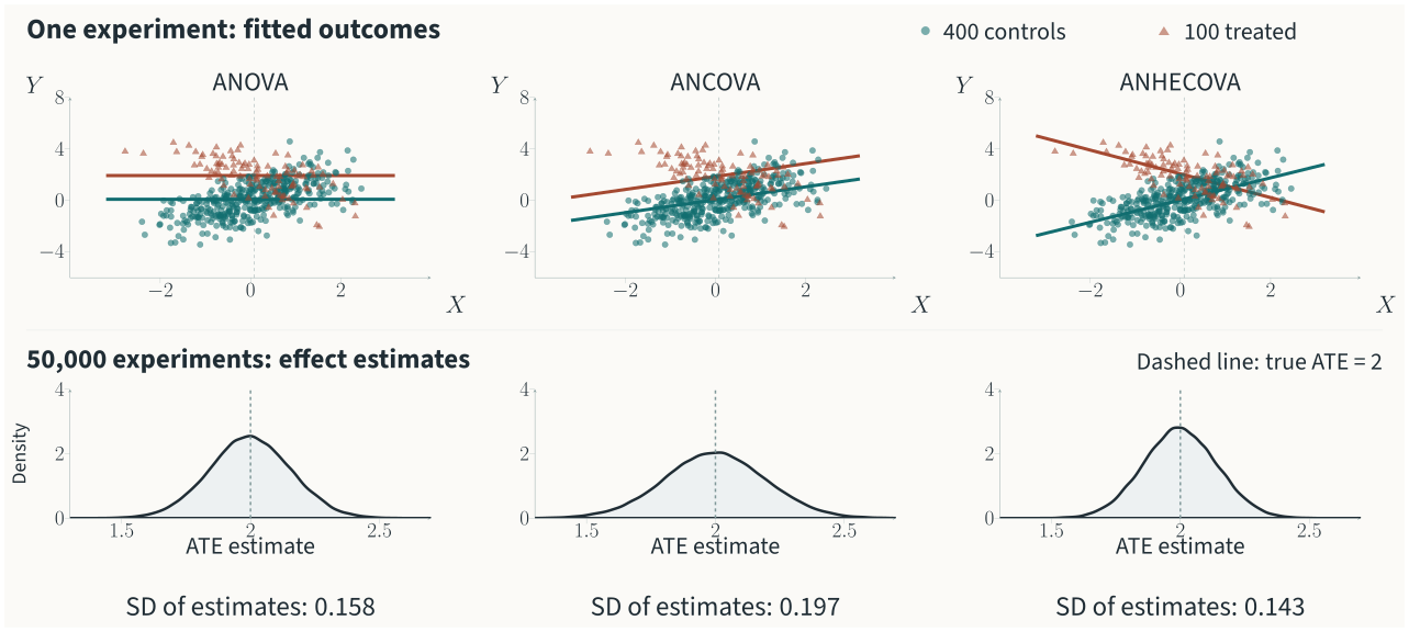
Compare fitted outcomes at the overall covariate mean \(\bar X\).

Method Least-squares fit Fitted lines
ANOVA \(Y\sim1+A\) Horizontal
ANCOVA \(Y\sim1+A+X\) Parallel
ANHECOVA \(Y\sim1+A+(X-\bar X)+A(X-\bar X)\) Separate slopes

ANCOVA: analysis of covariance. ANHECOVA: analysis of heterogeneous covariance.

Adjustment: parallel slopes

Potential outcomes: \(Y(0)=X+\epsilon_0\), \(Y(1)=2+X+\epsilon_1\).

Top: the same experiment, with 400 controls and 100 treated units, fitted three ways. Bottom: distributions of the three ATE estimators over 50,000 new experiments, on common axes with true ATE 2 marked. Standard deviations are 0.157, 0.112 and 0.112.

Adjustment: opposing slopes

Potential outcomes: \(Y(0)=X+\epsilon_0\), \(Y(1)=2-X+\epsilon_1\).

The same random draws and assignments as the parallel-slopes example, changing only the treated slope. Top: fitted outcomes. Bottom: sampling distributions of ATE estimates, with standard deviations 0.158 for ANOVA, 0.197 for ANCOVA and 0.143 for ANHECOVA.

1. Blocking

Fisher’s seven-by-seven Latin-square stained-glass window at Gonville and Caius College, photographed by Schutz in 2006. Glass by Maria McClafferty.

Compare treatments within groups of similar units.

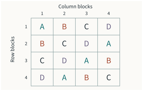
Four-by-four Latin square: four row blocks and four column blocks, with treatments A, B, C and D each appearing once per row and column.

Latin square: a special fractional factorial design.

  • Block on two factors.
  • Each treatment, once per row.
  • Each treatment, once per column.
  • Randomize within these constraints.

Fisher (1926), The arrangement of field experiments; The Design of Experiments (1935), ch. V. Caius window: Maria McClafferty; photo Schutz (2006), straightened by McGeddon, CC BY-SA 2.5.

Fisher was a controversial figure. Further reading and talks: Gonville & Caius College, Fisher in the 21st Century.

1. Blocking: the same simulation

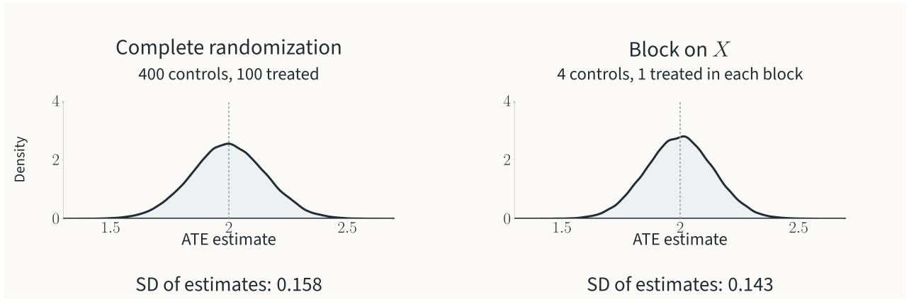
Opposing slopes: \(Y(0)=X+\epsilon_0\), \(Y(1)=2-X+\epsilon_1\).

Each new sample: sort by \(X\); form 100 blocks of five. Assign one treated unit and four controls per block; estimate by difference in means.

Sampling distributions of the unadjusted ATE estimate across 50,000 new experiments with opposing slopes. The complete-randomization baseline is exactly the ANOVA result on slide 5. Blocking treats one unit in each covariate block of five. Both use the same axes and mark the true ATE at 2; standard deviations are 0.158 and 0.143.

2. Stepped wedge design: An example

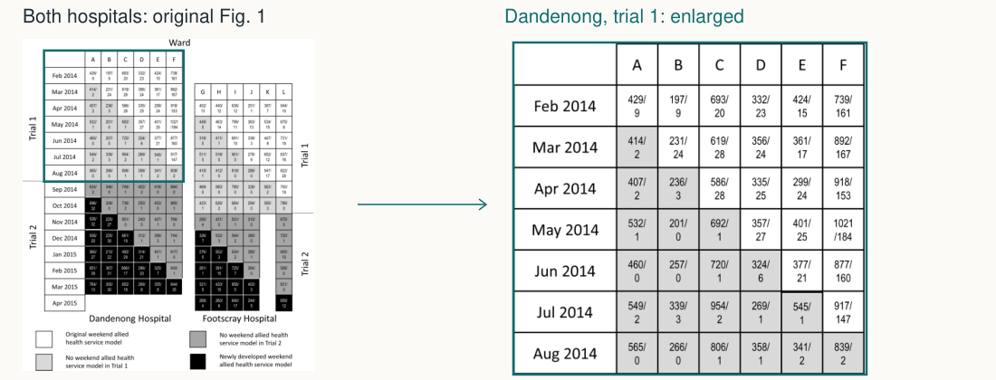
Original Fig. 1 shows both Dandenong and Footscray hospitals and both trials. A teal box highlights Dandenong trial 1; the right panel enlarges that part. White cells retain the original weekend allied health service model; light grey cells have services withdrawn.

Cell counts: weekday / weekend allied-health service occasions.

Six wards · 7,986 admissions · outcome: log(patient length of stay).

Haines et al. (2017), Impact of disinvestment from weekend allied health services…, Fig. 1, CC BY; highlight and enlarged crop added. Reanalysis: Zhang and Zhao (2023), §2.

2. Stepped wedge design: Assignment and exposure

Assignment: \(Z_w\) is the crossover month for ward \(w\).

\[Z\text{ is uniform over the }6!=720\text{ permutations of }(2,3,4,5,6,7).\]

Exposure: patient \(i\) enters ward \(w_i\) in month \(t_i\).

\[A_i(Z)=\mathbf 1\{t_i\ge Z_{w_i}\}\qquad(1=\text{weekend service withdrawn}).\]

  • Sharp null: all outcomes stay fixed under every schedule.
  • Randomization test: change the cross-over order; recompute exposure and statistic.

Zhang and Zhao (2023), What is a randomization test?, §§2–3.

2. Stepped wedge design: Randomization tests

Statistic: the exposure coefficient in \(Y\sim1+A\), or \(Y\sim1+A+\text{ward}\).

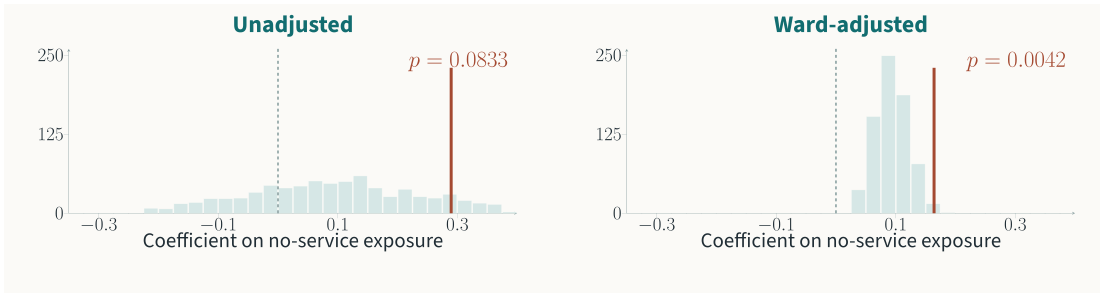
Exact distributions of the unadjusted and ward-adjusted coefficients over 720 schedules. Rust lines mark the observed coefficients, 0.290 and 0.164. Upper-tail p-values are 60/720 and 3/720.

Observed coefficients: 0.290 and 0.164. Rust lines mark the observations.

One-sided sharp-null tests: \(p=60/720\) and \(p=3/720\).

Recalculated from Haines et al. (2017), S2 Data. Zhang and Zhao (2023), §2, Table 1.

3. Group sequential design: Multiple testing

Can we stop an experiment early if the result is “clearly” statistically significant already?

  • The multiple hypothesis testing problem.
  • Family-wise error rate.
  • Bonferroni’s correction.

3. Group sequential design: Repeated testing

Independent \(Y_i\sim N(\mu,1)\); \(P_k=1-\Phi(T_k)\); \(k=1,2,\ldots,5\).

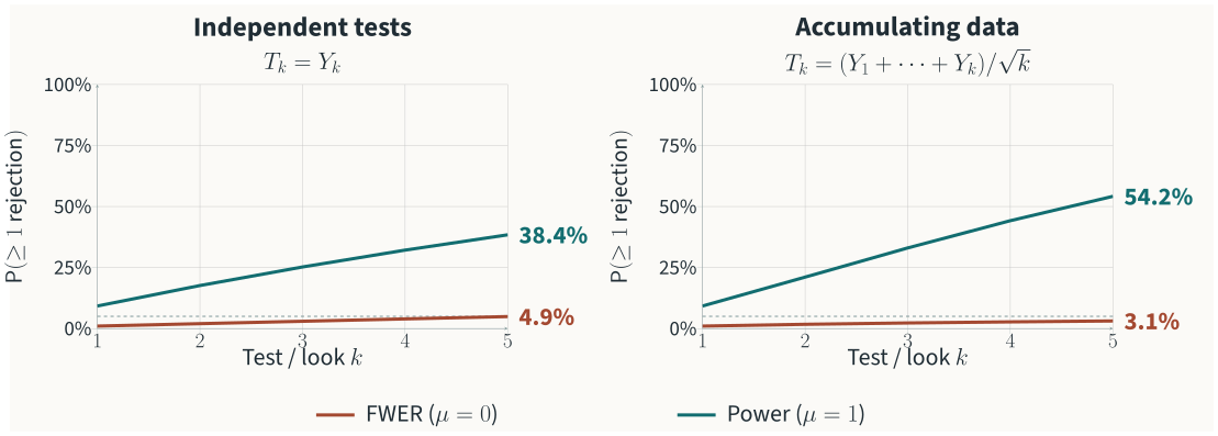
Probability of at least one rejection by test or look k, for k from 1 to 5. Left: independent tests with Bonferroni at 1% per test. Right: accumulating data with the same Bonferroni cutoff. Each panel shows rust FWER at mean zero and teal power at mean 1 on the same 0–100% probability axis. At five tests or looks, FWER is 4.9% and 3.1%; power is 38.4% and 54.2%. Shared legend; deterministic normal calculations.

Bonferroni: reject when \(P_k\le0.05/5\).

3. Group sequential design: Alpha-spending function

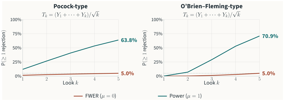
Independent \(Y_i\sim N(\mu,1)\); \(H_0:\mu\le0\); \(T_k=(Y_1+\cdots+Y_k)/\sqrt{k}\).

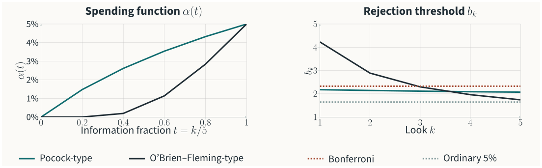
Left: Pocock-type and O’Brien–Fleming-type cumulative spending functions alpha(t), both reaching 5% at information fraction one. Right: the corresponding rejection thresholds b_k against look k, with ordinary 5% and Bonferroni reference thresholds. Reject at the first T_k greater than or equal to b_k. O’Brien–Fleming-type spending requires stronger early evidence.

Spending: \(\operatorname{\mathsf{P}}_0\{\max_{j\le k}(T_j-b_j)\ge0\}=\alpha(k/5)\), \(\alpha(1)=0.05\).

3. Group sequential design: Type I error and power

Independent \(Y_i\sim N(\mu,1)\); \(H_0:\mu\le0\); \(k=1,2,\ldots,5\).

Cumulative probability of at least one rejection by look k for the same five-look accumulating-data experiment. Left: Pocock-type. Right: O’Brien–Fleming-type. Each panel shows rust FWER at mean zero and teal power at mean 1 on the same 0–100% probability axis, with a dashed 5% reference. Both rules finish at 5% FWER. Pocock-type has more power at looks 1 to 4; O’Brien–Fleming-type overtakes at look 5 and finishes at 70.9%, versus 63.8%. Deterministic normal calculations.

4. Enrichment designs: FOURIER trial

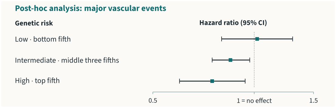
Evolocumab (PCSK9 inhibitor) versus placebo; overall primary-endpoint hazard ratio 0.85.

Post-hoc genetic analysis of FOURIER, with the endpoint major vascular events. Corrected hazard ratios for low, intermediate and high genetic risk are 1.02 (0.80–1.30), 0.85 (0.75–0.97) and 0.75 (0.60–0.94). One enlarged forest plot shows all three confidence intervals on a log-ratio axis, with a no-effect line at one.

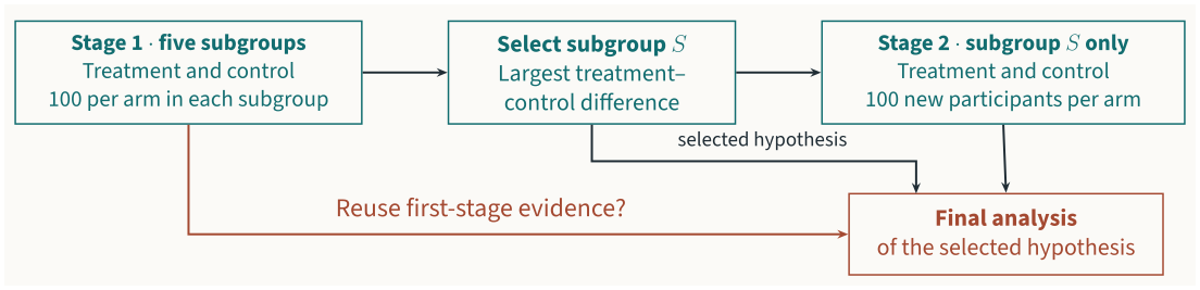
Possible enrichment: recruit broadly → select subgroup → concentrate recruitment.

Results redrawn: Sabatine et al. (2017), Evolocumab and Clinical Outcomes…; Marston et al. (2020), Predicting Benefit From Evolocumab Therapy…, Fig. 2, corrected 2024.

4. Enrichment designs: Selecting a subgroup

  • One treatment; five prespecified subgroups, with treatment effects \(\beta_j\).
  • Independent normal outcomes, variance 1; larger is better. Test \(H_S:\beta_S\le0\).

Stage 1 randomizes 100 to treatment and 100 to control within each of five disjoint subgroups. Select subgroup S with the largest first-stage treatment-control difference. Stage 2 recruits only subgroup S and randomizes 100 new participants per arm. Arrows show how selection and first-stage evidence can enter the final analysis.

4. Enrichment designs: Simulation results.

Nominal one-sided level: 5% · Probabilities calculated by numerical integration.

Rejection probability (%) Pooled \(z\) Bonferroni–
Bonferroni
Stage 2 \(z\) only Selective \(z\)
Effects \((0,0,0,0,0)\)
Marginal false rejection 16.6 4.9 5.0 5.0
Effects \((0.3,0,0,0,0)\)
Marginal false rejection 5.2 2.0 0.9 0.9
False rejection given \(S\in\{2,3,4,5\}\) 28.2 10.6 5.0 5.0
Power given \(S=1\) 95.3 73.7 68.3 69.7
Effects \((0.3,-0.3,-0.3,-0.3,-0.3)\)
Power given \(S=1\) 91.5 70.6 68.3 88.5