Lecture 2: Randomization and Experimental Design

Causal Inference and Statistical Designs · Michaelmas 2026 · Qingyuan Zhao

Randomization makes population inference possible

• Review: Neyman–Rubin model, \(A_i(z)=z_i\), and randomization.
• Difference-in-means estimator and its randomization distribution.

Example: Moderna’s COVID vaccination trial.

Does vaccination prevent symptomatic COVID-19?

Random assignment (1:1 within strata) → two injections, 28 days apart → follow-up

Per-protocol population

Group	Cases	Total	Risk
mRNA-1273	11	14,134	0.078%
Placebo	185	14,073	1.315%

Risk ratio:
0.078% / 1.315% = 5.92%.

Fisher’s exact test in R

> tab <- rbind(vaccine = c(11, 14123),
               placebo = c(185, 13888))
> fisher.test(tab)
p-value < 2.2e-16
95 percent confidence interval:
 0.02866549 0.10715476
sample estimates:
odds ratio
0.05846475

Baden et al. (2021; online 30 December 2020), Efficacy and Safety of the mRNA-1273 SARS-CoV-2 Vaccine, Fig. 1 and primary efficacy results; open full text. R documentation: Fisher’s Exact Test for Count Data.

Randomization: three roles

1. Avoid hidden bias.
   Random assignment and causal identification.
2. Justify analysis of variance.
   Analysis of variance (ANOVA), covariate adjustment, increase precision by design.
3. Construct exact tests.
   Use the experiment’s actual assignment distribution.

Cox (2009), Randomization in the Design of Experiments, §2, p. 416.

Role 1: Avoid hidden bias

Theorem (Identification). Consider i.i.d. units in the Neyman–Rubin model with pre-treatment \(X\) and binary exposure \(A\). Assume \(A\independent\{Y(0),Y(1)\}\mid X\) and \(0<\operatorname{\mathsf{P}}(A=1\mid X)<1\). Then the population ATE is identified by

\[\begin{aligned} \operatorname{\mathsf{E}}\{Y(1)-Y(0)\} &=\operatorname{\mathsf{E}}\!\left\{\operatorname{\mathsf{E}}(Y\mid A=1,X)-\operatorname{\mathsf{E}}(Y\mid A=0,X)\right\}\\[0.5em] &=\operatorname{\mathsf{E}}\!\left\{\frac{AY}{\operatorname{\mathsf{P}}(A=1\mid X)} -\frac{(1-A)Y}{\operatorname{\mathsf{P}}(A=0\mid X)}\right\}. \end{aligned}\]

Right-most quantity is called inverse-probability weighting (IPW).

Role 2: Justify ANOVA inference

Analysis of variance

Source	Sum of squares	d.f.	Mean square	\(F\)-statistic
Treatment	\(S_A\)	\(1\)	\(S_A\)	\(\dfrac{S_A}{S_E/(n-2)}\)
Residual	\(S_E\)	\(n-2\)	\(S_E/(n-2)\)	—
Total	\(S_T\)	\(n-1\)	—	—

• Justification under independent Gaussian errors with equal variance.

Randomization justifies ANOVA mean squares

Theorem. Consider a completely randomized (\(n_1\) out of \(n\)) experiment. Under the sharp null, \(Y_i(1)=Y_i(0)\) for all \(i\), we have

\[\operatorname{\mathsf{E}}(S_A\mid Y(\cdot)) =S^2 \quad \text{and} \quad \operatorname{\mathsf{E}}(S_E\mid Y(\cdot)) =(n-2) S^2,\]

where \(S^2=S_0^2=S_1^2\) is the sample variance of \(Y_1(0), \dots, Y_n(0)\).

• Equal expected mean squares without assuming Gaussian outcomes.

Cox (2009), Randomization in the Design of Experiments, §3.2. Ding and Dasgupta (2018), A randomization-based perspective on analysis of variance….

Fisher’s geometric intuition

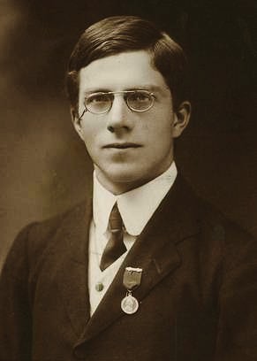
Ronald Aylmer Fisher in 1913; photographer unknown.

“He could picture the distribution of n results as a pattern in n-dimensional space, and he could see that randomization would produce a symmetry in that pattern rather like that produced by a kaleidoscope, and which approximated the required spherical symmetry available, in particular, from standard normal theory assumptions.”

— Joan Fisher Box (1980)

Box (1980), R. A. Fisher and the Design of Experiments, 1922–1926. Portrait: unknown photographer (1913), public domain.

Role 3: Construct exact tests

Fisher’s exact test and randomization inference

• Two binomials: fixed group sizes; condition on total cases.
• Sharp null: imputation and exact validity.
• Randomization distribution: use the actual assignment law.

Zhang and Zhao (2023), What is a randomization test?, §§1.3, 3, 5.1; open preprint.

Covariate adjustment for completely randomized experiments

Compare fitted outcomes at the overall covariate mean \(\bar X\).

Method	Least-squares fit	Fitted lines
ANOVA	\(Y\sim1+A\)	Horizontal
ANCOVA	\(Y\sim1+A+X\)	Parallel
ANHECOVA	\(Y\sim1+A+(X-\bar X)+A(X-\bar X)\)	Separate slopes

ANCOVA: analysis of covariance. ANHECOVA: analysis of heterogeneous covariance.

Reluga, Ye and Zhao (2022), A unified analysis of regression adjustment in randomized experiments, §§2–3.

Adjustment: parallel slopes

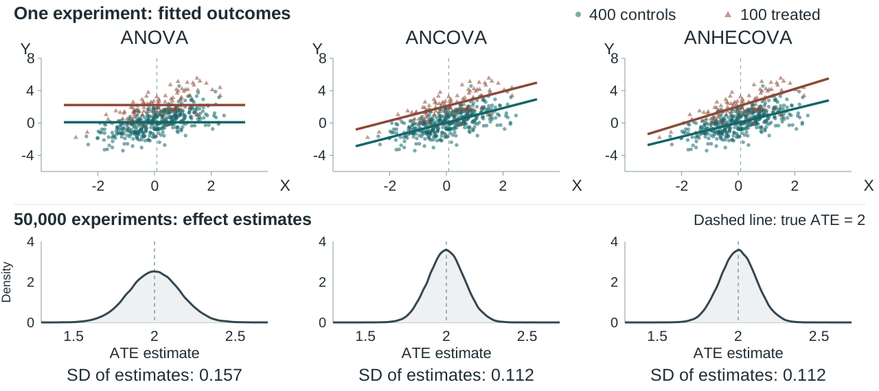
Potential outcomes: \(Y(0)=X+\epsilon_0\), \(Y(1)=2+X+\epsilon_1\).

Top: the same experiment, with 400 controls and 100 treated units, fitted three ways. Bottom: distributions of the three ATE estimators over 50,000 new experiments, on common axes with true ATE 2 marked. Standard deviations are 0.157, 0.112 and 0.112.

Adjustment: opposing slopes

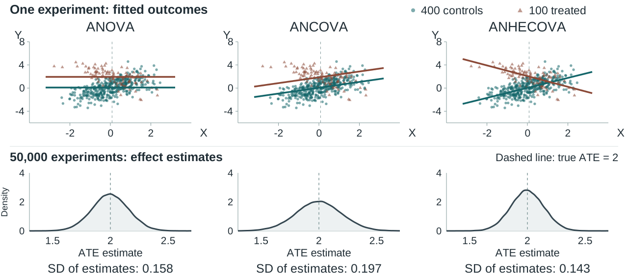
Potential outcomes: \(Y(0)=X+\epsilon_0\), \(Y(1)=2-X+\epsilon_1\).

The same random draws and assignments as the parallel-slopes example, changing only the treated slope. Top: fitted outcomes. Bottom: sampling distributions of ATE estimates, with standard deviations 0.158 for ANOVA, 0.197 for ANCOVA and 0.143 for ANHECOVA.

Blocking

Fisher’s seven-by-seven Latin-square stained-glass window at Gonville and Caius College, photographed by Schutz in 2006. Glass by Maria McClafferty.

Compare treatments within groups of similar units.

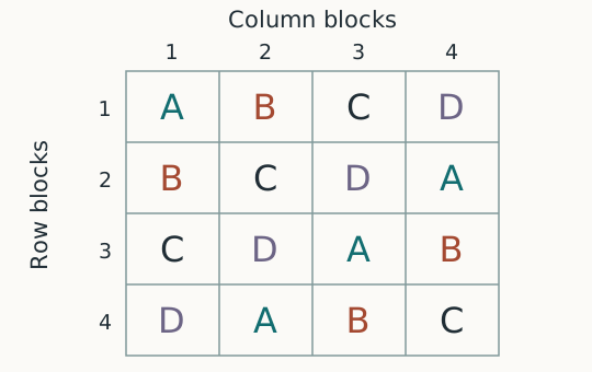
Four-by-four Latin square: four row blocks and four column blocks, with treatments A, B, C and D each appearing once per row and column.

Latin square

• Block on two factors.
• Each treatment, once per row.
• Each treatment, once per column.
• Randomize within these constraints.

Fisher (1926), The arrangement of field experiments; The Design of Experiments (1935), ch. V. Caius window: Maria McClafferty; photo Schutz (2006), straightened by McGeddon, CC BY-SA 2.5.

Further reading and talks: Gonville & Caius College, Fisher in the 21st Century.

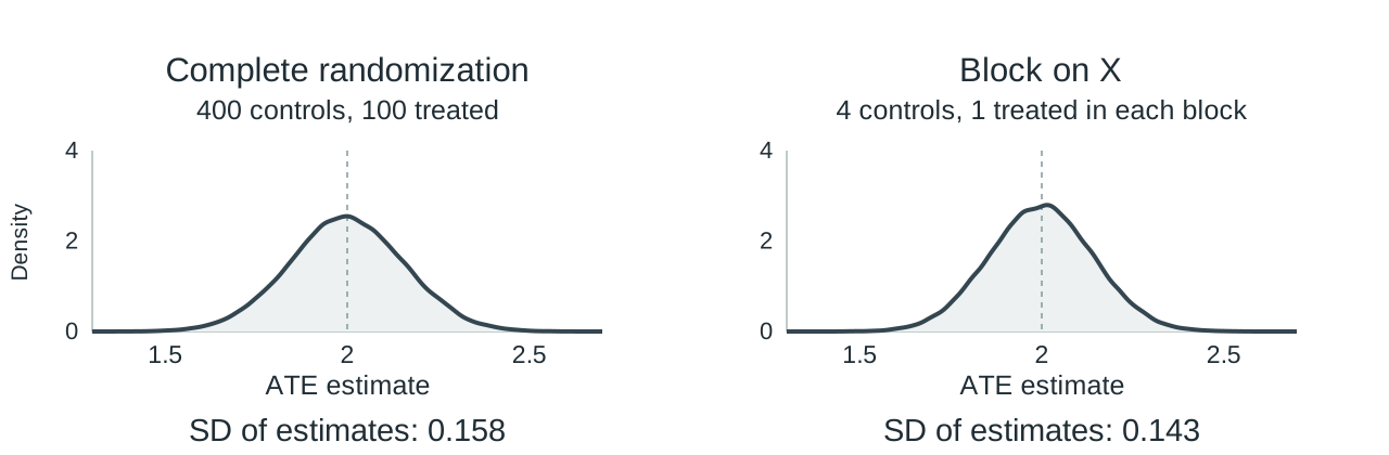
Blocking: the same simulation

Opposing slopes: \(Y(0)=X+\epsilon_0\), \(Y(1)=2-X+\epsilon_1\).

Each new sample: sort by \(X\); form 100 blocks of five. Assign one treated unit and four controls per block; estimate by difference in means.

Sampling distributions of the unadjusted ATE estimate across 50,000 new experiments with opposing slopes. The complete-randomization baseline is exactly the ANOVA result on slide 12. Blocking treats one unit in each covariate block of five. Both use the same axes and mark the true ATE at 2; standard deviations are 0.158 and 0.143.